A controller has three possible actions, with values 1.0, 0.8, and 0.0. If those numbers were perfectly known and only immediate reward mattered, choosing the first action every time would be sensible. Why pay the controller to do anything else?
The maximum-entropy objective behind Soft Actor-Critic adds a temperatureThe coefficient that trades expected reward against policy entropy.-weighted policy entropyA measure of how spread out a policy’s action probabilities are. to expected reward. Its soft policy-improvement step favors an exponential distribution over action values; practical SAC approximates the relevant values and policy with learned functions. This changes the optimization problem, rather than merely adding noise after solving the original one. The SAC paper, Sections 3.2–4.2.
SAC uses this entropy-regularized idea inside an off-policy actor-critic algorithm and evaluates it on continuous-control tasks. Its policy and critic are learned approximations; a finite softmax over three known actions is an exactly solvable view of the objective, not the continuous-action algorithm or an explanation of all its empirical performance.
Put a price on diversity
Consider our deliberately smaller problem: one state, one decision, three known rewards. Let the action probabilities be p₁, p₂, p₃. We maximize
J(p) = Σ pᵢqᵢ − α Σ pᵢ log(pᵢ)
subject to probabilities summing to one. Natural logarithms measure entropy in nats. The coefficient α therefore exchanges reward units for nats. Differentiating with a multiplier for the probability constraint gives qᵢ − α(log pᵢ + 1) + λ = 0. Rearranging and normalizing yields pᵢ = exp(qᵢ/α) / Σ exp(qⱼ/α).
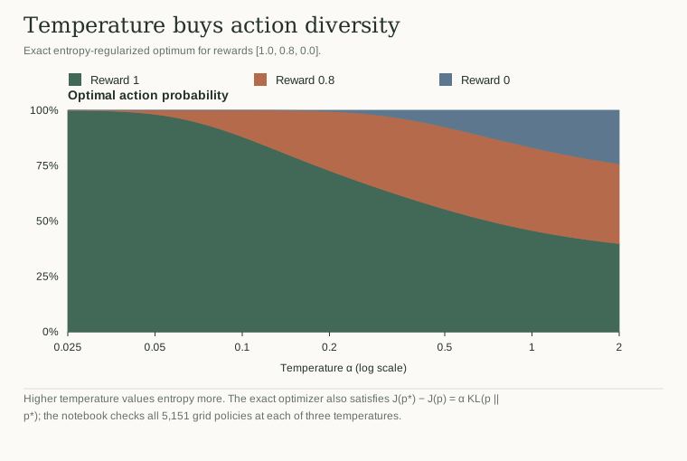
The particularly revealing expression is the ratio p₁/p₂ = exp((1.0 − 0.8)/α). At α = 0.2, the better action receives approximately 2.72 times the probability of the runner-up. At α = 0.05, that ratio is about 54.6. Nothing in this calculation requires either action to be unexplored. Randomization is desirable because the stated objective explicitly values it.
An exact calculation, not a training curve
The accompanying Python illustration evaluates that distribution for three temperatures. It also calculates expected reward, entropy, and the combined objective, and checks the result against deterministic and uniform policies. It contains no critic learning, replay buffer, or continuous-control simulator: it isolates the choice that an entropy term makes attractive.
Subtracting the largest value before exponentiation keeps the calculation numerically well behaved without changing any probabilities. The common factor cancels between numerator and denominator. This small implementation detail matters when α is small: exponentiating a large positive number can overflow even though the final probability is perfectly ordinary.
Read the output columns separately. Expected reward and the entropy-augmented objective answer different questions. A policy can improve the second while sacrificing the first. The stacked probability chart makes the trade visible: the zero-value action gains noticeable mass only when diversity has become valuable enough under the entropy-weighted objective to outweigh part of its reward disadvantage. That is not a mistake in the optimizer; it is the optimizer following the specification.
Change the units before changing the algorithm
Now multiply every reward by ten while leaving α fixed. The exponential ratios become much sharper. Multiplying α by ten as well restores the original probabilities. Our final assertion checks exactly this invariance. Reporting a temperature without reporting reward scaling therefore leaves an important part of the experiment unspecified.
For a follow-up learning experiment, record ordinary return and policy entropy separately, use equal interaction budgets, and compare several training seeds. An entropy bonus might help a learner discover useful behavior, but this exact one-step calculation cannot establish faster learning or greater robustness. It establishes the more basic fact that “more unpredictable” and “better under the chosen objective” can describe the same policy.
A numerical certificate for the optimum
The extended experiment does more than compare the softmax policy with two hand-picked alternatives. For each of α = 0.05, 0.2, and 1, it evaluates all 5,151 three-action probability vectors on the hundredth grid. None exceeds the exact optimum. More usefully, every comparison satisfies J(p) − J(p) = α KL(p ∥ p) within 10⁻¹².
The identity follows from log pᵢ = qᵢ/α − log Z. Substituting it into the divergence gives αΣpᵢlog(pᵢ/pᵢ) = αΣpᵢlog pᵢ − Σpᵢqᵢ + αlog Z. Since the optimum has value αlog Z, the expression is exactly the objective gap. Nonnegative KL divergence therefore certifies the optimum for every probability vector, not only the grid. The exhaustive grid checks the implementation of that identity.
The figure sweeps temperature continuously on a logarithmic axis. The stacked areas are probabilities and sum to one at every point; reward and entropy remain separate fields in the data. This avoids placing unlike units on a shared vertical axis or making the entropy bonus look like additional task reward.
The practical lesson is to audit the entire objective. Reward scaling, entropy units, and temperature jointly specify which distributions are attractive. Randomness is not necessarily uncertainty, and an entropy-seeking policy is not necessarily confused. It may be the exact optimizer of a deliberately different objective.