A training dashboard can look better while the model takes longer to reach its target. The missing quantity is how much progress each processed example buys. If a larger batch mostly repeats information the optimizer already has, higher examples per second may not compensate for more expensive updates.
Pollux combines system throughput with statistical efficiencyHow much learning progress is obtained from the examples processed. in its goodputTraining throughput adjusted for how much useful learning the processed examples provide. model. It uses observations during training to coordinate resource allocation and training configuration, rather than treating GPU count and batch size as unrelated decisions. The relevant distinction is useful learning progress versus data processed, not a blanket preference for small batches. Pollux paper
Pollux's published evaluation reports 37–50% lower average job completion time than its comparison schedulers across the evaluated real jobs and trace-driven workloads. That is a cluster-level result: the scheduler has to make progress estimates useful enough to guide allocations while jobs and training conditions change. The scalar experiment below asks a smaller prerequisite question: can a throughput-only ranking be wrong even when the update arithmetic is perfectly correct?
A deliberately simple counterexample
Take the scalar objective L(w) = w²/2 and start at w = 1. Every training example is identical and has gradient w. Averaging 64 copies or 1,024 copies therefore produces exactly the same gradient. With learning rate 0.25, each update multiplies w by 0.75.
After n updates, the loss is 0.5 × 0.75^(2n). Reaching loss at most 0.0001 requires 15 updates. Batch size does not change that count because this construction has no sampling noise to reduce.
Now introduce an explicitly invented timing model: an update costs 0.01 seconds of fixed overhead plus batch_size / 10,000 seconds of processing. With batch 64, an update takes 0.0164 seconds and processes about 3,902 examples/s. With batch 1,024, an update takes 0.1124 seconds and processes about 9,110 examples/s.
The larger batch wins the throughput chart by more than a factor of two. Yet its 15 updates take 1.686 modeled seconds, compared with 0.246 for the smaller batch. It also consumes 15,360 examples instead of 960. Both reach the same scalar loss with the same update rule.
What this calculation does and does not establish
The accompanying code performs the actual scalar updates but uses modeled time rather than a stopwatch. That distinction matters: Python overhead on a laptop would not validate the assumed accelerator cost model. The example is intentionally extreme so the mechanism is unambiguous. Extra examples contain zero new gradient information.
Real stochastic gradients are different. Averaging additional examples can reduce noise, enable a different learning rate, and change the number of updates required. The favorable batch size can also change during training. A comparison that freezes an unsuitable learning rate at one batch size may measure poor tuning rather than an intrinsic scheduling limit.
For an empirical study, record both data processed and optimizer updates. Choose the validation target before the comparison, include runs that never reach it, and keep the tuning budget comparable. A throughput number without the target, learning-rate schedule, and quality outcome is insufficient to rank training configurations.
The useful question for a scheduler is whether another unit of resource shortens the path to the agreed target enough to justify its cost. The miniature counterexample gives that question a concrete failure case; it does not estimate Pollux's cluster-level gains.
When noise makes the extra examples useful
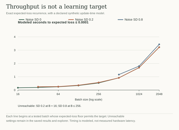
The extended notebook replaces identical gradients with an exact expected-loss recurrence. Each example has gradient w plus independent, zero-mean noise with variance σ². Averaging B examples gives noise variance σ²/B. At learning rate η, the second moment therefore follows E[w²]ₜ₊₁ = (1 − η)² E[w²]ₜ + η²σ²/B. This is an analytical expectation calculation, not a noisy single-seed training run. It assumes that the gradient noise is independent of the current weight and that its variance stays fixed.
With η = 0.25, the expected loss has a floor of σ²/(14B). A target at or below that floor cannot be reached from the stated initial condition in finite time. The notebook marks those configurations as unreachable rather than assigning them a favorable running time or silently excluding them.
Across the eight tested batches, the fastest modeled configuration changes from B = 16 without noise to B = 32 at σ = 0.2 and B = 512 at σ = 0.8. Their times to expected loss 0.0001 are 0.1740, 0.2508, and 1.1628 seconds respectively. These are not three comparable hardware measurements: they are three different statistical problems evaluated under one explicit cost model. Within each problem, every candidate receives the same target and update rule.
This creates a useful test for a scheduler's objective. A rule that always selects the largest batch fails in the noise-free case. A rule that always selects the smallest batch cannot reach the target in the high-noise case. Useful progress depends jointly on throughput and the learning dynamics; neither component can be optimized in isolation. A deployed system must estimate that relationship from observed training rather than being handed this recurrence.