Two jobs each need three CPU units. They cannot run together on a four-CPU machine, even if plenty of memory is free. A third job needs only one CPU unit but three memory units. It may be the missing complement. Resource scheduling is not a single queue ordered by a single size.
DeepRM frames multi-resource scheduling as sequential action selection. The agent can place several jobs before advancing simulated time. Its slowdown objective assigns each unfinished job a per-timestep cost equal to the inverse of its duration. With undiscounted rewards, the accumulated cost equals the sum of job slowdowns. DeepRM, Sections 3.2–3.4.
DeepRM's initial experiments report scheduling performance comparable to strong heuristics and adaptation to changed conditions. Its learned policy is trained against a specified objective, rather than rewarded for visual packing density alone. The small schedules below make the objective's accounting inspectable before any policy training enters the picture.
Three jobs reveal two different choices
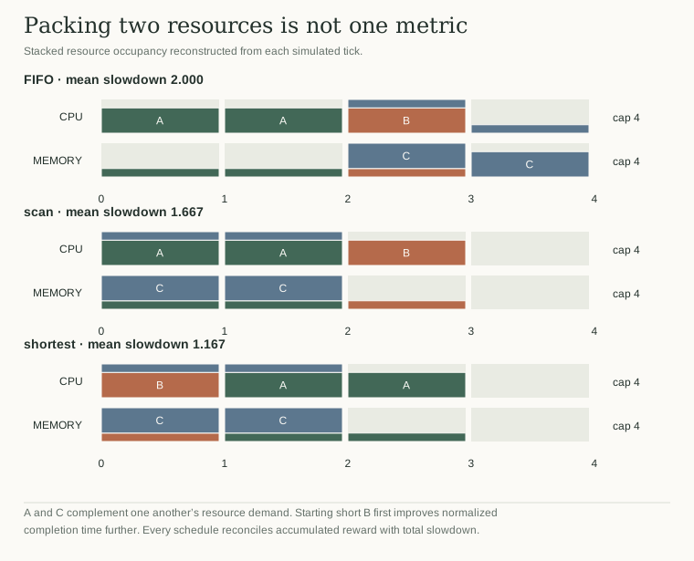
Our example has capacity (CPU=4, memory=4). All jobs arrive at time zero. Job A needs (3,1) for two ticks; B needs (3,1) for one tick; C needs (1,3) for two ticks. Resources are reserved throughout execution. There is no preemption and no uncertainty about duration.
A strict FIFO policy starts A. It then encounters B, which cannot fit beside A, and stops looking. C could fit but waits behind B. At time two, B and C start together. Completion times are A=2, B=3, C=4. Dividing by durations gives slowdowns 1, 3, and 2, for a mean of 2.
A scanning policy keeps looking past the blocked B and starts C alongside A. Both finish at time two; B finishes at time three. Its mean slowdown is (1 + 3 + 1)/3, approximately 1.667. The improvement comes from a concrete change in occupied resource rectangles, not from a mysterious benefit of learning.
But scanning is not the whole objective. A shortest-duration order starts B with C. When B finishes at time one, A fits beside the still-running C. Completion times become A=3, B=1, C=2, producing mean slowdown (1.5 + 1 + 1)/3, approximately 1.167. Delaying A slightly improves the normalized completion time of B substantially.
Audit the reward, not just the schedule
The executable simulator implements these three explicit rules; it does not train a policy. Before each tick passes, it adds −1/duration for every unfinished job, including waiting jobs. It records finish times and independently calculates total slowdown afterward. An assertion checks that the negative accumulated reward matches that total.
This identity is a useful environment test. Job j contributes one charge for every tick between its arrival and completion. Therefore its cumulative charge is exactly its time in the system divided by its duration. Accidentally charging only running jobs would make every job contribute one, eliminating the incentive to reduce waiting. Charging only waiting jobs would instead remove the service-time contribution; that is a different accounting convention, though related for fixed jobsets.
The figure shows CPU and memory occupancy on the same tick scale. A and C have complementary resource demands. Mean slowdown is reported beside each schedule because utilization and normalized completion time describe different properties.
The next meaningful test would change the job mix and arrival times while preserving identical inputs across policies. A learned scheduler would need held-out job sequences and explicit training budgets. These three handcrafted jobs establish the mechanics of feasibility and reward accounting; they do not demonstrate that a trained policy generalizes or that one heuristic always wins.
Sweep both capacities and audit every schedule
The extension varies CPU and memory capacity independently from three through six units. For each of the sixteen capacity combinations, it evaluates every permutation of the three jobs under the scanning rule. The recorded best order is the best of those six scan priorities, not a claim to have solved arbitrary online scheduling. Ties are retained by the underlying data, even though one representative order is displayed.
Increasing only one capacity can leave the other resource as the binding constraint. At the original (4, 4) point, complementary jobs share both resources efficiently, but ordering still changes slowdown. The CPU and memory panels use the same tick boundaries and are reconstructed directly from active-job sets. A rectangle's height is its resource demand; the empty portion is unused capacity.
Every simulated tick asserts feasibility in both dimensions. Every finished schedule then independently checks that cumulative per-tick reward equals negative total slowdown. Those are different invariants: a feasible scheduler can still have an incorrect reward implementation, and a correct reward accumulator can still describe an infeasible schedule. Checking both catches errors that a plausible-looking mean can conceal.
A stronger evaluation would add held-out arrivals and duration errors, then compare policies under the same trace. Before that, this tiny suite is a useful regression test for an environment: a blocked head-of-line job must not silently erase a later feasible choice, and waiting jobs must remain in the slowdown charge.