A sender receives a congestion mark. Should it reduce its sending window just as much when one packet in a hundred is marked as when every packet is marked? A binary event says congestion exists. A sequence of marked and unmarked packets contains information about its extent.
DCTCP marks packets above a queue threshold and conveys the marked fraction back to the sender. The sender smooths that fraction into α and uses cwnd × (1 − α/2) for a congestion response, rather than always halving the window. Other TCP mechanisms remain part of the protocol. DCTCP, Section 3.1.
The DCTCP paper reports the same or better throughput than TCP with 90% less buffer space in its evaluated 1- and 10-Gbps environment. That is a closed-loop transport result. The component test below verifies its estimator and reduction equations before making any claim that a prescribed mark sequence actually improves short-flow completion.
Work through the estimator
Let F be the fraction marked in the latest observation window. The update is α_new = (1 − g)α_old + gF, where g controls the weight assigned to the latest observation. For our original arithmetic example, initialize α to zero and set g to 1/16.
If the next marked fraction is 0.25, α becomes 0.015625. A 100-packet congestion window would then be reduced by only 0.78125 packets. The reduction is not 12.5 packets, which would follow from substituting the unsmoothed fraction directly. Keeping F and α in separate columns prevents that easy implementation mistake.
Now observe a fully marked window. The new estimate becomes approximately 0.077148. Applied to the already reduced window, it causes a stronger reduction. A later unmarked observation makes α decay, but it does not itself constitute a new marked-ACK congestion event.
The illustrative code therefore updates the estimator every round and reduces the window only in rounds with marks. It allows at most one reduction in each synthetic round. It deliberately omits additive increase, slow start, loss recovery, ACK timing, and queue evolution, so the resulting window trace is a component calculation, not a complete transport flow.
Smoothing buys memory and costs responsiveness
The second run repeats exactly the same marked-fraction sequence with g = 0.5. Larger g makes the estimate move farther toward each new observation. It also forgets old observations more rapidly. Neither choice is automatically better: the useful balance depends on how quickly the condition changes and how noisy the observations are.
For a constant fraction f, repeated updates have the exact form αₖ = f + (α₀ − f)(1 − g)^k. The final check compares the recurrence with this expression for f = 0.4. This is a deterministic test of the estimator, independent of any story about a datacenter workload.
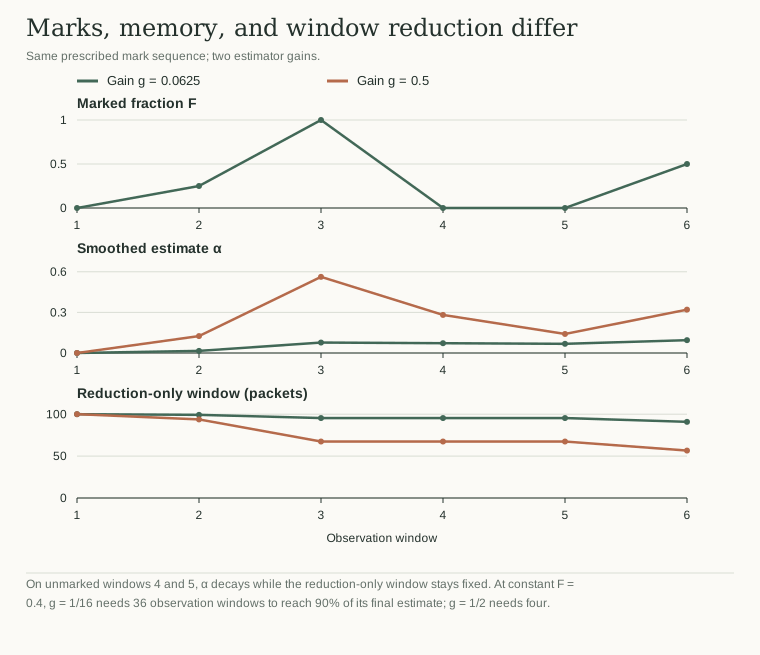
The figure aligns F, α, and congestion window on separate axes. The rounds without marks distinguish the estimator from the response: the estimate changes there while this isolated reduction component leaves the window unchanged.
What this does and does not say about short requests
A shorter standing queue can reduce the time a small response spends behind a large transfer, but our prescribed F values do not establish that a queue actually shrinks. That requires closing the loop: the window affects packet arrivals, arrivals affect queues and marks, and feedback arrives after delay.
A next simulation could add one bottleneck and both long and short flows, then compare completion times as well as throughput. Keep initial conditions and traffic identical. The present example verifies the numerical feedback mechanism that such a simulator would need; it does not claim a reproduction of the paper's network experiments.
Measure estimator memory in observation windows
For a constant marked fraction f and initial α = 0, the response is αₖ = f[1 − (1 − g)ᵏ]. Reaching 90% of the final value therefore requires ceil(log 0.1 / log(1 − g)) observation windows. The extension checks this prediction against 256 recurrence updates for each of four gains.
At g = 1/64, the response takes 147 windows. At the illustrative 1/16 setting it takes 36; at 1/4 it takes nine; at 1/2 it takes four. The corresponding half-life at 1/16 is about 10.74 windows. These are estimator timescales, not milliseconds: converting them to time requires the duration and definition of the actual observation windows.
The main figure aligns three quantities without mixing their units: the prescribed marked fraction, the smoothed estimate, and the reduction-only congestion window. In unmarked windows four and five, α decays while the plotted window remains unchanged. The estimator remembers past congestion, but that memory is not itself a new marked-ACK event in this isolated calculation.
A larger gain reacts faster to the step and also to noise. Which tradeoff is useful depends on the feedback process, the round-trip delay, and the traffic. To answer the article's application question about short requests, the next model must let window changes influence arrivals and queues, then let those queues generate the marks. Without that loop, a window trace is evidence about an equation, not about latency improvement.