From Camera Pixels to a Bird’s-Eye Grid

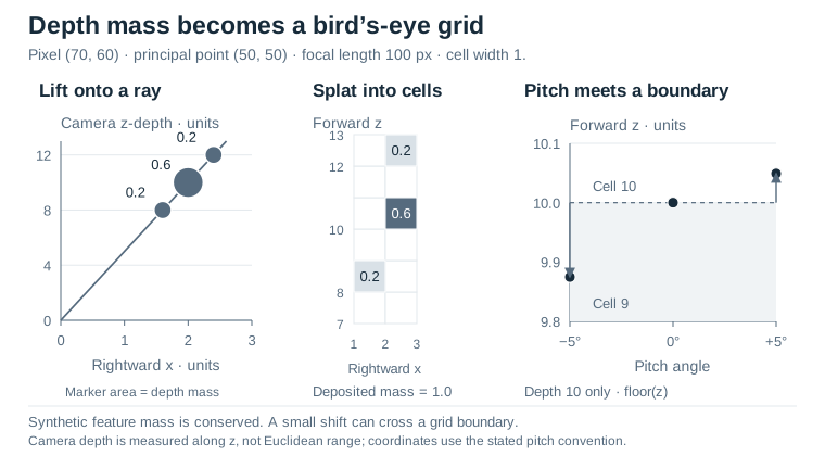
A pixel does not identify a ground-plane location

A feature at one image coordinate tells us a direction from the camera, not a unique three-dimensional point. Near and far objects can occupy the same pixel. A bird's-eye mapA top-down representation that places observations into a shared map-like coordinate frame. needs a position, so an image-based system must handle that missing depth information before it can accumulate evidence in map cells.

Lift, Splat, Shoot, Section 3, predicts a depth distribution and contextual feature for each image location. It distributes the feature along a camera ray, transforms those points into a shared frame, and pools them into bird's-eye pillars. Its learned components and downstream planning are outside this example. One hand-authored ray makes the coordinate transform and accumulation explicit.

State the axes before writing the formula

Use camera coordinates with x right, y down, and z forward. For image coordinate (u, v), focal length f, principal point (cx, cy), and depth d measured along camera z, unprojection gives x=(u-cx)d/f, y=(v-cy)d/f, and z=d. This is not Euclidean range along a unit ray; confusing those depth conventions changes every projected point.

The example pixel is (70, 60), with principal point (50, 50) and focal length 100 pixels. At z-depth 10, its camera point is (2, 1, 10). Depths 8 and 12 instead produce (1.6, 0.8, 8) and (2.4, 1.2, 12). A fixed image offset therefore creates larger lateral displacement at greater depth.

The fixture assigns those three depth hypotheses weights 0.2, 0.6, and 0.2. It rotates the y–z coordinates by a stated pitch angle, then keeps x and rotated z as the two map coordinates. This explicit convention makes the sign testable: z_world = sin(pitch)*y + cos(pitch)*z. A real camera rig also needs translation and a consistent world-frame definition; neither is silently inferred here.

Splatting is accumulation, not choosing one answer

Each transformed point deposits its weight in the grid cell found by flooring its coordinates divided by cell width. When multiple points share a cell, their weights add. The total deposited mass remains one as long as no point is discarded. That conservation check is a useful unit test independent of whether the assumed depth distribution is correct.

The program prints cell coordinates and accumulated mass for several grid widths and pitch angles. A finer grid distinguishes nearby hypotheses but can reveal sharper changes under a small calibration perturbation. A coarser grid may hide the coordinate error by placing both points in the same cell. Stable cell identity is therefore not proof of accurate geometry.

The three weighted ray samples separate two effects. Depth uncertainty spreads feature mass along the ray; pitch changes where those samples land in the grid. The cells contain synthetic feature mass, not calibrated probabilities that physical space is occupied.

For the depth-ten sample, positive five-degree pitch shifts forward position by only 0.0491 units and leaves the tested cell indices unchanged. Negative five-degree pitch moves samples across the nearby integer boundaries. The asymmetric cell result comes from quantization boundaries, not asymmetric uncertainty.

Separate the errors you are investigating

Depth quantization, uncertain depth, camera calibration, and map resolution are different mechanisms. Change one at a time, then inspect interactions. In particular, rounding a depth estimate to a bin is not the same experiment as spreading a distribution over several bins. A trained perception model can adapt its features to its training setup, but this geometric illustration makes no claim about that adaptation or about driving accuracy.

import math
from collections import defaultdict

u, v = 70.0, 60.0
cx, cy, focal = 50.0, 50.0, 100.0
depths = ((8.0, 0.2), (10.0, 0.6), (12.0, 0.2))

def lift(depth, pitch_degrees):
    x = (u-cx)*depth/focal
    y = (v-cy)*depth/focal
    z = depth
    angle = math.radians(pitch_degrees)
    world_z = math.sin(angle)*y + math.cos(angle)*z
    return x, world_z

def splat(cell_width, pitch):
    grid = defaultdict(float)
    for depth, mass in depths:
        x, z = lift(depth, pitch)
        cell = (math.floor(x/cell_width), math.floor(z/cell_width))
        grid[cell] += mass
    assert abs(sum(grid.values())-1.0) < 1e-12
    return [(cell, round(mass, 3)) for cell, mass in sorted(grid.items())]

for width in (1.0, 2.0):
    for pitch in (0.0, 5.0, -5.0):
        print('width', width, 'pitch', pitch, 'cells', splat(width, pitch))
base = lift(10.0, 0.0)
tilted = lift(10.0, 5.0)
print('depth10_forward_shift', round(tilted[1]-base[1], 4))
assert base == (2.0, 10.0)

width 1.0 pitch 0.0 cells [((1, 8), 0.2), ((2, 10), 0.6), ((2, 12), 0.2)]
width 1.0 pitch 5.0 cells [((1, 8), 0.2), ((2, 10), 0.6), ((2, 12), 0.2)]
width 1.0 pitch -5.0 cells [((1, 7), 0.2), ((2, 9), 0.6), ((2, 11), 0.2)]
width 2.0 pitch 0.0 cells [((0, 4), 0.2), ((1, 5), 0.6), ((1, 6), 0.2)]
width 2.0 pitch 5.0 cells [((0, 4), 0.2), ((1, 5), 0.6), ((1, 6), 0.2)]
width 2.0 pitch -5.0 cells [((0, 3), 0.2), ((1, 4), 0.6), ((1, 5), 0.2)]
depth10_forward_shift 0.0491