Network congestion control
The Bandwidth–Delay Product Knee
A single-bottleneck model separates the inflight data that sustains throughput from the extra data that adds queueing delay.
A sender doubles the amount of unacknowledged data. Sometimes throughput doubles. Sometimes throughput barely moves and round-trip time grows instead. The difference is whether the path needed more data to remain busy or was already full.
The original BBR paper models a path using bottleneck bandwidth and round-trip propagation time. It estimates these quantities from delivery-rate and RTT observations and probes because measurements depend on the operating point. Its idealized inflight diagram distinguishes underfilled, bandwidth-limited, and buffer-limited regions. BBR, “Congestion and Bottlenecks” and “Characterizing the Bottleneck”.
Specify the units before doing the multiplication
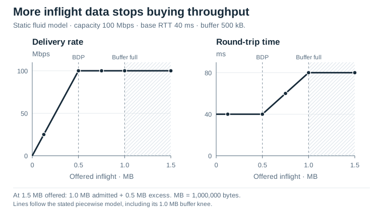
The illustrative fluid model has a 100-megabit-per-second bottleneck and 40 milliseconds of base round-trip time. Dividing by eight converts capacity to 12.5 million bytes per second. Multiplying by 0.04 seconds gives a bandwidth-delay product of 500,000 bytes.
That number is the model's useful inflight scale. With only 125,000 bytes circulating, the sender can deliver 125,000 / 0.04 = 3,125,000 bytes per second, or 25 Mbps. It does not supply enough outstanding data to sustain the full 100-Mbps bottleneck. At 500,000 bytes, the same calculation reaches capacity.
Now raise inflight to 750,000 bytes. The extra 250,000 bytes form a modeled queue. Draining them at 12.5 million bytes per second takes 20 milliseconds, so RTT becomes 60 milliseconds. Delivered throughput remains 100 Mbps. The sender is buying latency, not additional steady-state capacity.
Add a finite buffer explicitly
Give the bottleneck another 500,000 bytes of buffer capacity beyond the bandwidth-delay product. The largest admitted inflight amount in this simplified model is therefore one million bytes. A hypothetical offered amount of 1.5 million bytes exceeds that limit by 500,000. The script reports those excess bytes separately rather than silently allowing an unlimited queue.
This is a static fluid calculation, not a packet simulation. “Excess bytes” is an instantaneous capacity-accounting quantity here, not a measured loss rate, retransmission volume, or amount dropped by an actual BBR implementation. The code has no feedback state machine and does not compare congestion-control algorithms.
For admitted data, it calculates queue delay, RTT, and delivery rate, then checks a useful identity: admitted inflight divided by modeled RTT equals delivery rate. Below the knee, RTT remains at the base value. Above it, inflight and RTT rise together while delivery rate stays fixed. The assertion connects the two regimes instead of relying only on a plausible-looking graph.
Why a single observation is ambiguous
An observed delivery rate of 25 Mbps could mean a 25-Mbps bottleneck. In this example it instead means that a 100-Mbps path is underfilled. Likewise, an RTT of 60 milliseconds could reflect a longer base path or a 40-millisecond path with 20 milliseconds of queueing. The quantities become easier to separate when observations span different operating points.
The two boundaries are 500,000 bytes, where throughput reaches capacity, and one million bytes, where the buffer also fills. Between them, extra inflight data increases RTT without increasing delivery rate. Both boundaries follow from the stated capacity, propagation time, and buffer size.
Changing capacity, competing flows, and delayed feedback make online estimation harder than this fixed-parameter calculation. The model isolates the throughput and queueing relationship described in the 2016 paper; it does not simulate BBR's feedback loop or establish how current BBR versions behave.
Run the example
The Python 3 example uses only the standard library. The notebook, source, figure data and recorded output are included in the complete bundle.
Inspect the code and recorded output
capacity_bps = 100_000_000
capacity_bytes_s = capacity_bps / 8
base_rtt_s = 0.040
buffer_bytes = 500_000
bdp_bytes = capacity_bytes_s * base_rtt_s

def model(offered_bytes):
    admitted = min(offered_bytes, bdp_bytes + buffer_bytes)
    excess = offered_bytes - admitted
    queued = max(admitted - bdp_bytes, 0.0)
    rtt = base_rtt_s + queued / capacity_bytes_s
    delivery = min(capacity_bytes_s, admitted / base_rtt_s)
    assert abs(admitted / rtt - delivery) < 1e-6
    assert queued <= buffer_bytes and excess >= 0
    return delivery * 8 / 1e6, rtt * 1000, queued, excess

print(f"BDP={bdp_bytes:.0f} bytes; buffer={buffer_bytes} bytes")
observations = []
for offered in [125_000, 500_000, 750_000, 1_500_000]:
    rate, rtt, queue, excess = model(offered)
    observations.append((rate, rtt))
    print(f"offered={offered:7d} rate={rate:6.1f}Mbps RTT={rtt:5.1f}ms "
          f"queue={queue:.0f} excess={excess:.0f} bytes")

assert max(rate for rate, _ in observations) == 100.0
assert min(rtt for _, rtt in observations) == 40.0
print("Static fluid-model consistency checks: passed")
Recorded CPU output
BDP=500000 bytes; buffer=500000 bytes
offered= 125000 rate=  25.0Mbps RTT= 40.0ms queue=0 excess=0 bytes
offered= 500000 rate= 100.0Mbps RTT= 40.0ms queue=0 excess=0 bytes
offered= 750000 rate= 100.0Mbps RTT= 60.0ms queue=250000 excess=0 bytes
offered=1500000 rate= 100.0Mbps RTT= 80.0ms queue=500000 excess=500000 bytes
Static fluid-model consistency checks: passed