Four devices do not guarantee four devices' worth of useful work at every instant. In a pipeline, later stages wait for earlier outputs, and earlier stages eventually wait for the batch to drain. Microbatches create more opportunities to overlap that work, but they cannot repair an arbitrarily slow stage.
GPipe partitions sequential layers into stages, splits a mini-batch into microbatches, and accumulates gradients before one synchronous update. The paper combines this schedule with recomputation to manage activation memory. Its bubble analysis motivates increasing the microbatch count relative to pipeline depth. GPipe paper
GPipe's evaluation includes a 557-million-parameter AmoebaNet reaching 84.4% ImageNet top-1 accuracy. Its contribution is not just an idle-time formula: synchronous gradient accumulation and activation re-materialization make a large partitioned network trainable. A bubble calculation can illuminate the schedule, but it does not capture that model-quality or memory result.
Start with a balanced pipeline
Assume four stages and a one-unit forward operation for each microbatch at every stage. The first microbatch needs four units to traverse the pipeline. Each subsequent microbatch finishes one unit later. For m microbatches, forward completion therefore takes m + 3 units.
For this illustration, backward operations cost the same as forward operations. All forward work completes before the backward pipeline starts, and the backward pipeline runs in the reverse stage order. Total time is 2(m + 3). Each stage performs 2m units of useful work, so average utilization is m/(m + 3).
With one microbatch, utilization is 25%. With four, it is approximately 57.1%. With sixteen, it is approximately 84.2%. The bubble has not vanished; it has been amortized over more work.
These comparisons keep per-microbatch duration fixed, meaning total batch work increases with m. For a fixed-size mini-batch, microbatches become smaller instead. The same idealized utilization ratio can follow if duration scales perfectly with size, but actual kernels need not obey that assumption.
Put one slow stage in the middle
Now assign stage durations [1, 1, 2, 1]. Every microbatch needs five units of forward work, but the second microbatch cannot emerge only one unit after the first. The slow stage sets a two-unit cadence.
The forward makespan becomes 2m + 3. Including the separate backward wave gives 4m + 6. Sixteen microbatches now take 70 time units, while aggregate useful work is 160 stage-time units. Across four stages, utilization is 160/(4 × 70), approximately 57.1%.
Even with very many microbatches, utilization approaches 62.5%, not 100%. Each microbatch requires five units of total stage work, but the bottleneck permits only one microbatch every two units across a four-stage system. Increasing m cannot change that imbalance.
The code uses a small dependency recurrence: each operation starts after both its incoming microbatch and its stage are available. It models no communication, recomputation, optimizer cost, or memory pressure. Its output describes the declared schedule, not measured GPipe throughput.
For a real partition, measure stage times at the intended microbatch size rather than balancing parameter counts alone. Activation sizes and recomputation can make two equal-sized parameter groups behave differently. Batch-dependent operations also require care when deciding what numerical equivalence means.
Fix the total batch work, then charge for each operation
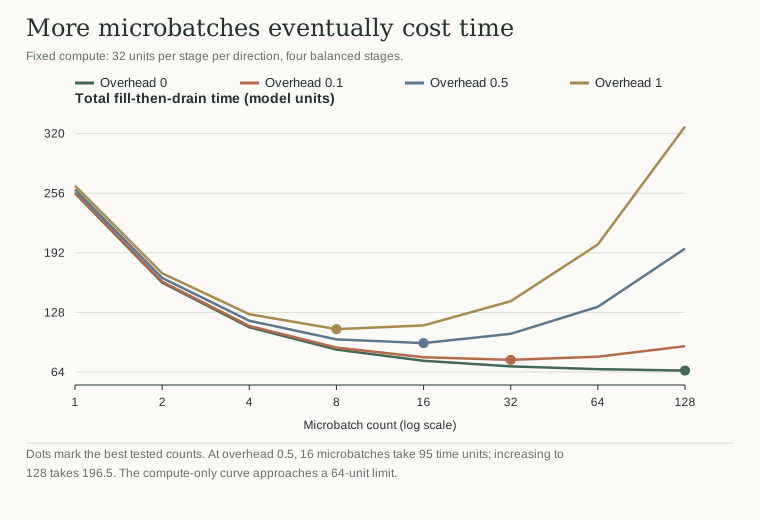
The extended experiment keeps 32 units of compute at each stage in each direction. Splitting that work into m microbatches gives a stage operation duration of 32/m + h, where h is a fixed per-operation overhead. This keeps compute constant while making the overhead cost of finer splitting explicit. The same fill-then-drain recurrence yields total time 2(m + 3)(32/m + h).
Expanding the expression exposes the tradeoff: 64 + 192/m + 2hm + 6h. The first term is the ideal compute time. The second shrinks as the pipeline bubble is amortized. The third grows because every added microbatch incurs more overhead. For h > 0, the continuous optimum is m = √(96/h); a real implementation must choose an admissible integer count and obey batch-size constraints.
With h = 0.5, the best tested power-of-two count is 16 and elapsed time is 95 units. At 128 microbatches it rises to 196.5 units. At zero overhead, the tested curve keeps improving and approaches 64 units. There is no contradiction: the assumptions changed, and the notebook records them alongside every result.
The figure therefore holds useful compute fixed and plots elapsed time, rather than treating a higher utilization number as sufficient. Its overhead model is deliberately simple. To turn it into a planning tool, measure the full stage-duration curve at each intended microbatch size, including communication and recomputation. Then rerun the dependency recurrence. Dividing one large-batch measurement by m would assume away exactly the small-kernel behavior this test is meant to expose.