A simulated controller can choose a conservative action or an aggressive action. The aggressive action earns more reward but also incurs more cost. Is subtracting a sufficiently large penalty from reward equivalent to imposing a cost budget? Even the smallest example reveals a distinction worth keeping explicit.
Constrained Policy Optimization starts from a constrained Markov decision process: maximize expected reward while keeping expected discounted auxiliary costs below specified limits. Its practical algorithm uses approximate trust-region updates rather than solving every candidate policy exactly. These are constraints on expected cost, not promises that every trajectory avoids harm. CPO, Sections 4–6.
CPO develops a policy-performance bound involving policy divergence and uses it to construct approximate constrained trust-region updates. Its simulated locomotion evaluations concern constrained learning, while the one-step problem here solves the feasible set exactly. The distinction helps separate an objective-specification issue from the additional approximation errors of a learning algorithm.
Solve one decision completely
Our synthetic problem has one state and terminates immediately after an action. The conservative action earns reward 4 and cost 0. The aggressive action earns reward 10 and cost 3. Let p be the probability of choosing the aggressive action. Expected reward is 4 + 6p; expected cost is 3p.
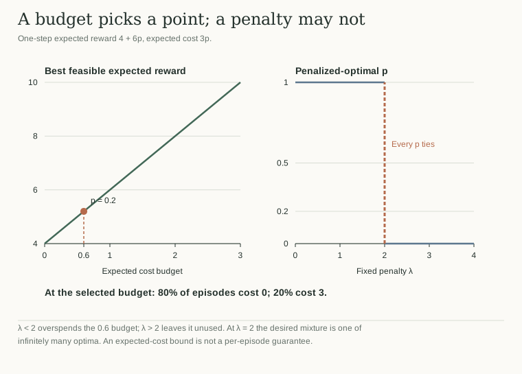
Set the budget to 0.6. The feasible interval is 0 ≤ p ≤ 0.2. Reward increases throughout that interval, so the constrained optimum is p = 0.2, with reward 5.2 and cost 0.6. Randomization matters: the best feasible deterministic policy has reward only 4. The 20% mixture improves the expectation while exactly using the budget.
The feasible region is a line segment: increasing p moves reward from 4 toward 10 and cost from zero toward three. The budget ends that segment at p = 0.2. The figure compares this budget-selected operating point with the alternatives selected by a fixed penalty.
What a fixed penalty selects
Replace the constraint with the objective reward − λ × cost. Substituting our expressions gives 4 + (6 − 3λ)p. If λ is below 2, the optimizer selects p = 1 and exceeds the budget. If λ is above 2, it selects p = 0 and leaves usable budget unspent. At λ = 2, every mixture has exactly the same penalized score. The desired p = 0.2 is among the optima, but the penalty alone does not single it out.
This example does not establish that penalty methods can never solve constrained problems. It demonstrates a narrower engineering problem: a coefficient can encode a tradeoff without uniquely encoding the desired operating point. An optimizer's tie-breaking and a method for selecting or adapting the multiplier may matter.
The executable illustration enumerates probabilities in hundredth increments. It identifies the best feasible policy and reports the full interval of penalized maximizers for several λ values. Because the exact solution lies on this grid, enumeration and the algebra agree. The assertions check both feasibility and the reward calculation; there is no approximate policy-gradient training hidden behind the table.
Read the budget literally
At the constrained optimum, 20% of episodes still take the action with cost 3. Expected cost 0.6 does not mean each episode costs at most 0.6. If cost represented a physical hazard, that distinction would be decisive. This remains a simulation-only example, not a controller specification for use around people.
A useful follow-up would change the requirement before changing the optimizer: compare an expectation budget, a bound on violation probability, and a strict action prohibition. Those are different tasks. Writing the requirement precisely is more informative than calling all three “safe” and hoping a large negative reward makes them interchangeable.
Trace the frontier instead of tuning one penalty
The notebook sweeps budgets from zero to three. The constrained optimum is p = budget/3 until the aggressive action can be chosen every time. Its reward frontier is 4 + 2 × budget. Each additional expected-cost unit buys two reward units in this model. The plot beside that frontier shows the penalized optimizer jumping from p = 1 to p = 0 as λ crosses two, with the entire interval optimal at the tie.
That geometry explains why a multiplier and a budget should not be treated as interchangeable user inputs. A multiplier sets the slope of an indifference line. A budget selects a location on the feasible frontier. Here the frontier is itself a straight line, so matching the slope creates indifference across all mixtures. Additional tie-breaking, primal feasibility checks, or an adaptive constrained procedure is needed to choose the desired point.
The saved data also records the full episode-cost distribution for the selected budget: probability 0.8 at cost zero and probability 0.2 at cost three. The expectation is 0.6, but every aggressive episode exceeds 0.6. For budgets below three, the probability of exceeding the budget equals p; at budget three it becomes zero because neither action exceeds the limit.
This last distinction is not a mathematical footnote. An expectation constraint, a chance constraint, and an action prohibition define different feasible policies. Writing one down and then reporting success under another would change the task. The exact example is useful as a specification and test case before introducing approximate gradients or real-world risk.