The cost of asking a learned index for a key
A nine-row reanalysis of Apple’s AMIPS timing table separates a promising component ratio from the end-to-end claim it cannot yet support.
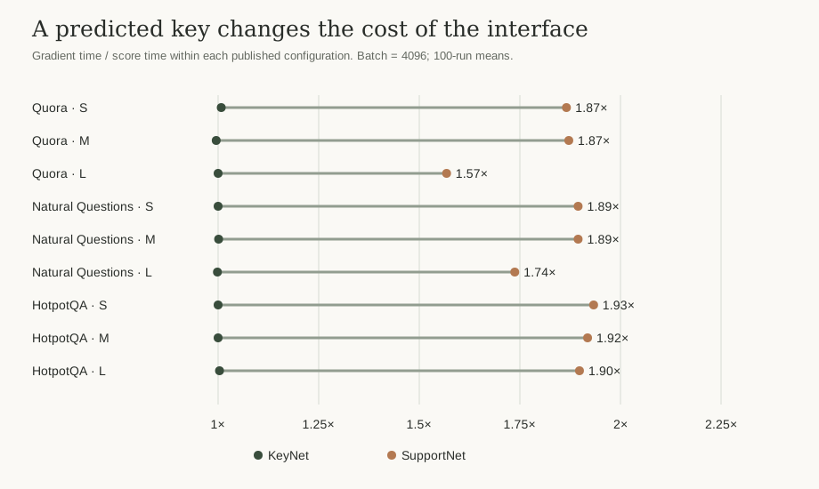
A learned retrieval model does not have a single inference cost. The useful output might be a scalar score that chooses a partition, or a vector that replaces the query sent to an index. Those interfaces ask different amounts of work from the same network. That distinction is visible in the published timings for Apple’s AMIPS research, before any attempt to reproduce the training pipeline.
Research question: how much does the requested output change the reported cost of SupportNet and KeyNet, and how much of that difference could survive once search is added back?
Read the interface before the stopwatch
For a fixed collection of key vectors, the maximum inner productFind the stored vector with the largest dot product with a query vector. is a support functionFor a direction, report the largest dot product achieved by any vector in a set.: it maps a query to the largest dot product against the database. Where that function is differentiable, its gradient is the maximizing key. At a tie, a unique gradient need not exist; the subgradient view is the appropriate mathematical description.
SupportNet models the scalar function. Recovering a predicted key therefore asks for differentiation with respect to the input. KeyNet predicts a key vector directly. For cluster routing, scalar scores can be sufficient; for query remapping, the vector is the useful output. Neither architecture has to be described as universally faster for that distinction to matter. The Apple paper page describes the two interfaces, and the released implementation separates embedding, target construction and training.
Nine rows, four timing columns
The input to this analysis is the complete nine-row Appendix A.1 timing table: three database sizes, three parameter fractions, and score/gradient timings for each architecture. The caption identifies 4,096 queries per batch, 384-dimensional embeddings and means over 100 runs. All values were transcribed exactly into the attached CSV, with only scientific notation expanded to decimals.
Section 4.1 refers to this table as timing “per sample,” while the detailed Table 1 caption specifies seconds per batch. This analysis follows the caption; the within-row ratios are unaffected by that source-unit inconsistency. Dividing by 4,096 produces a throughput-normalized cost per query, not the latency of one query arriving alone. The article therefore keeps batch timing as the primary unit. The timing description does not identify the hardware, and there are no run-level samples or variance columns in this extraction. No confidence intervals are manufactured from nine different configurations.
Within SupportNet, gradient time is 1.57–1.93 times score time. Within KeyNet, the same ratio is 0.995–1.008, essentially equal at the precision of the reported means. Comparing the two gradient columns, SupportNet takes 1.64–2.11 times KeyNet’s reported time. The median across these nine configurations is 2.047, a descriptive median, not a population estimate or an accuracy-matched speedup.
| Database | SupportNet gradient ms / batch | KeyNet gradient ms / batch | Ratio |
|---|---|---|---|
| Quora | 4.08 | 2.12 | 1.925× |
| Natural Questions | 16.20 | 7.69 | 2.107× |
| HotpotQA | 30.50 | 14.90 | 2.047× |
A surprising detail is worth preserving instead of smoothing away: for Quora and Natural Questions, every L-size timing column is lower than its M-size counterpart. These are eight adjacent decreases across four columns and two datasets. The table alone cannot tell us whether that reflects architecture choices, execution behavior or measurement variation. It does tell us not to fit a monotonic “larger model means proportionally longer” curve through these rows.
Put search back into the denominator
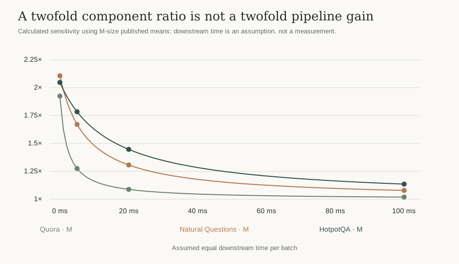
A component ratio disappears quickly when unchanged work dominates. Suppose the two mappings were followed by an equal downstream search cost D. With S denoting SupportNet’s reported gradient time and K denoting KeyNet’s, the combined ratio is:
This is a sensitivity calculation, not a measured pipeline. Equal downstream time and equal retrieval quality are assumptions; the table establishes neither. As D grows, the ratio tends toward one. Search cannot be silently omitted from an end-to-end claim, and an equal-probe comparison is not automatically an equal-recall comparison.
Explore the denominator
Choose a published mapping configuration and an assumed equal search time. The result is arithmetic, not a new benchmark.
Amortization needs a second accounting sheet
Training is a different denominator. If a learned path costs C more to prepare and saves Δt per served query at the required quality, a simple serial-compute break-even count is C / Δt. That expression is useful only when the costs share a unit and Δt is positive. Training on one device and serving on another requires monetary or resource weighting before adding their durations.
The nine timing rows supply neither training cost nor an accuracy-matched IVF baseline. They therefore cannot produce a numerical training break-even claim. The public repository’s three-stage pipeline makes the missing terms concrete: embedding, clustering and exact target construction precede network training. Key updates or query-distribution changes can force some of those costs to recur. A profitable static experiment is not yet a maintainable service.
A proper follow-up would pin the key set and query split, retain a held-out query distribution, and record query encoding, mapping, index search, reranking and result transfer separately. It would compare recall and total latency at matched targets, then account for index construction, learned-target generation, training and refresh frequency. Batch size and request-arrival behavior would remain explicit rather than being hidden behind a per-query average.
What this table changes
The strongest supported conclusion is narrow and useful: requesting a key vector adds a substantial relative cost to SupportNet’s published score interface, while KeyNet’s two reported interfaces cost about the same. That explains why the useful output belongs in a retrieval cost model. It does not establish which trained checkpoint is best, whether mapped search wins at a given recall, or how much a production system saves.
The attached analysis checks all nine configuration keys for uniqueness, positivity of timing values, the ratio bounds under added common work, and the eight non-monotonic size transitions. These checks protect the arithmetic and its interpretation. They do not turn paper means into independently measured hardware results.
Sources & reuse
- Olausson, Monteiro, Klein and Cuturi, Amortizing Maximum Inner Product Search with Learned Support Functions, version 1, Appendix A.1 / Table 1. The paper is CC BY 4.0. This article transforms the table into decimal CSV, ratios and new plots.
- Apple Machine Learning Research publication page, architectural context.
- Pinned AMIPS repository, pipeline context only. No Apple implementation code is redistributed here.
Recompute the nine timing rows
The included CSV preserves all four Table 1 timing columns. The notebook checks the nine configuration keys, regenerates the ratios and redraws the downstream-cost sensitivity using only the Python standard library.